Derivative of a function. Detailed theory with examples

Very easy to remember.

Well, let’s not go far, let’s immediately consider the inverse function. Which function is the inverse of the exponential function? Logarithm:

In our case, the base is the number:

Such a logarithm (that is, a logarithm with a base) is called “natural”, and we use a special notation for it: we write instead.

What is it equal to? Of course, .

The derivative of the natural logarithm is also very simple:

Examples:

1. Find the derivative of the function.
2. What is the derivative of the function?

Answers: The exponential and natural logarithm are uniquely simple functions from a derivative perspective. Exponential and logarithmic functions with any other base will have a different derivative, which we will analyze later, after we go through the rules of differentiation.

Rules of differentiation

Rules of what? Again a new term, again?!...

Differentiation is the process of finding the derivative.

That's all. What else can you call this process in one word? Not derivative... Mathematicians call the differential the same increment of a function at. This term comes from the Latin differentia - difference. Here.

When deriving all these rules, we will use two functions, for example, and. We will also need formulas for their increments:

There are 5 rules in total.

The constant is taken out of the derivative sign.

If - some constant number (constant), then.

Obviously, this rule also works for the difference: .

Let's prove it. Let it be, or simpler.

Examples.

Find the derivatives of the functions:

1. at a point;
2. at a point;
3. at a point;
4. at the point.

Solutions:

1. (the derivative is the same at all points, since it is a linear function, remember?);

Derivative of the product

Everything is similar here: let’s introduce a new function and find its increment:

Derivative:

Examples:

1. Find the derivatives of the functions and;
2. Find the derivative of the function at a point.

Solutions:

Derivative of an exponential function

Now your knowledge is enough to learn how to find the derivative of any exponential function, and not just exponents (have you forgotten what that is yet?).

So, where is some number.

We already know the derivative of the function, so let's try to reduce our function to a new base:

To do this, we will use a simple rule: . Then:

Well, it worked. Now try to find the derivative, and don't forget that this function is complex.

Happened?

Here, check yourself:

The formula turned out to be very similar to the derivative of an exponent: as it was, it remains the same, only a factor appeared, which is just a number, but not a variable.

Examples:
Find the derivatives of the functions:

Answers:

This is just a number that cannot be calculated without a calculator, that is, it cannot be written down in a simpler form. Therefore, we leave it in this form in the answer.

Note that here is the quotient of two functions, so we apply the corresponding differentiation rule:

In this example, the product of two functions:

Derivative of a logarithmic function

It’s similar here: you already know the derivative of the natural logarithm:

Therefore, to find an arbitrary logarithm with a different base, for example:

We need to reduce this logarithm to the base. How do you change the base of a logarithm? I hope you remember this formula:

Only now we will write instead:

The denominator is simply a constant (a constant number, without a variable). The derivative is obtained very simply:

Derivatives of exponential and logarithmic functions are almost never found in the Unified State Examination, but it will not be superfluous to know them.

Derivative of a complex function.

What is a "complex function"? No, this is not a logarithm, and not an arctangent. These functions can be difficult to understand (although if you find the logarithm difficult, read the topic “Logarithms” and you will be fine), but from a mathematical point of view, the word “complex” does not mean “difficult”.

Imagine a small conveyor belt: two people are sitting and doing some actions with some objects. For example, the first one wraps a chocolate bar in a wrapper, and the second one ties it with a ribbon. The result is a composite object: a chocolate bar wrapped and tied with a ribbon. To eat a chocolate bar, you need to do the reverse steps in reverse order.

Let's create a similar mathematical pipeline: first we will find the cosine of a number, and then square the resulting number. So, we are given a number (chocolate), I find its cosine (wrapper), and then you square what I got (tie it with a ribbon). What happened? Function. This is an example of a complex function: when, to find its value, we perform the first action directly with the variable, and then a second action with what resulted from the first.

In other words, a complex function is a function whose argument is another function: .

For our example, .

We can easily do the same steps in reverse order: first you square it, and I then look for the cosine of the resulting number: . It’s easy to guess that the result will almost always be different. An important feature of complex functions: when the order of actions changes, the function changes.

Second example: (same thing). .

The action we do last will be called "external" function, and the action performed first - accordingly "internal" function(these are informal names, I use them only to explain the material in simple language).

Try to determine for yourself which function is external and which internal:

Answers: Separating inner and outer functions is very similar to changing variables: for example, in a function

1. What action will we perform first? First, let's calculate the sine, and only then cube it. This means that it is an internal function, but an external one.
   And the original function is their composition: .
2. Internal: ; external: .
   Examination: .
3. Internal: ; external: .
   Examination: .
4. Internal: ; external: .
   Examination: .
5. Internal: ; external: .
   Examination: .

We change variables and get a function.

Well, now we will extract our chocolate bar and look for the derivative. The procedure is always reversed: first we look for the derivative of the outer function, then we multiply the result by the derivative of the inner function. In relation to the original example, it looks like this:

Another example:

So, let's finally formulate the official rule:

Algorithm for finding the derivative of a complex function:

It seems simple, right?

Let's check with examples:

Solutions:

1) Internal: ;

External: ;

2) Internal: ;

(Just don’t try to cut it by now! Nothing comes out from under the cosine, remember?)

3) Internal: ;

External: ;

It is immediately clear that this is a three-level complex function: after all, this is already a complex function in itself, and we also extract the root from it, that is, we perform the third action (put the chocolate in a wrapper and with a ribbon in the briefcase). But there is no reason to be afraid: we will still “unpack” this function in the same order as usual: from the end.

That is, first we differentiate the root, then the cosine, and only then the expression in brackets. And then we multiply it all.

In such cases, it is convenient to number the actions. That is, let's imagine what we know. In what order will we perform actions to calculate the value of this expression? Let's look at an example:

The later the action is performed, the more “external” the corresponding function will be. The sequence of actions is the same as before:

Here the nesting is generally 4-level. Let's determine the course of action.

1. Radical expression. .

2. Root. .

3. Sine. .

4. Square. .

5. Putting it all together:

DERIVATIVE. BRIEFLY ABOUT THE MAIN THINGS

Derivative of a function- the ratio of the increment of the function to the increment of the argument for an infinitesimal increment of the argument:

Basic derivatives:

Rules of differentiation:

The constant is taken out of the derivative sign:

Derivative of the sum:

Derivative of the product:

Derivative of the quotient:

Derivative of a complex function:

Algorithm for finding the derivative of a complex function:

1. We define the “internal” function and find its derivative.
2. We define the “external” function and find its derivative.
3. We multiply the results of the first and second points.

When deriving the very first formula of the table, we will proceed from the definition of the derivative function at a point. Let's take where x– any real number, that is, x– any number from the domain of definition of the function. Let us write down the limit of the ratio of the increment of the function to the increment of the argument at :

It should be noted that under the limit sign the expression is obtained, which is not the uncertainty of zero divided by zero, since the numerator does not contain an infinitesimal value, but precisely zero. In other words, the increment of a constant function is always zero.

Thus, derivative of a constant functionis equal to zero throughout the entire domain of definition.

Derivative of a power function.

The formula for the derivative of a power function has the form , where the exponent p– any real number.

Let us first prove the formula for the natural exponent, that is, for p = 1, 2, 3, …

We will use the definition of derivative. Let us write down the limit of the ratio of the increment of a power function to the increment of the argument:

To simplify the expression in the numerator, we turn to the Newton binomial formula:

Hence,

This proves the formula for the derivative of a power function for a natural exponent.

Derivative of an exponential function.

We present the derivation of the derivative formula based on the definition:

We have arrived at uncertainty. To expand it, we introduce a new variable, and at . Then . In the last transition, we used the formula for transitioning to a new logarithmic base.

Let's substitute into the original limit:

If we recall the second remarkable limit, we arrive at the formula for the derivative of the exponential function:

Derivative of a logarithmic function.

Let us prove the formula for the derivative of a logarithmic function for all x from the domain of definition and all valid values ​​of the base a logarithm By definition of derivative we have:

As you noticed, during the proof the transformations were carried out using the properties of the logarithm. Equality is true due to the second remarkable limit.

Derivatives of trigonometric functions.

To derive formulas for derivatives of trigonometric functions, we will have to recall some trigonometry formulas, as well as the first remarkable limit.

By definition of the derivative for the sine function we have .

Let's use the difference of sines formula:

It remains to turn to the first remarkable limit:

Thus, the derivative of the function sin x There is cos x.

The formula for the derivative of the cosine is proved in exactly the same way.

Therefore, the derivative of the function cos x There is –sin x.

We will derive formulas for the table of derivatives for tangent and cotangent using proven rules of differentiation (derivative of a fraction).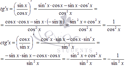

Derivatives of hyperbolic functions.

The rules of differentiation and the formula for the derivative of the exponential function from the table of derivatives allow us to derive formulas for the derivatives of the hyperbolic sine, cosine, tangent and cotangent.

Derivative of the inverse function.

To avoid confusion during presentation, let's denote in subscript the argument of the function by which differentiation is performed, that is, it is the derivative of the function f(x) By x.

Now let's formulate rule for finding the derivative of an inverse function.

Let the functions y = f(x) And x = g(y) mutually inverse, defined on the intervals and respectively. If at a point there is a finite non-zero derivative of the function f(x), then at the point there is a finite derivative of the inverse function g(y), and . In another post .

This rule can be reformulated for any x from the interval , then we get .

Let's check the validity of these formulas.

Let's find the inverse function for the natural logarithm (Here y is a function, and x- argument). Having resolved this equation for x, we get (here x is a function, and y– her argument). That is, and mutually inverse functions.

From the table of derivatives we see that And .

Let’s make sure that the formulas for finding the derivatives of the inverse function lead us to the same results:

As you can see, we got the same results as in the derivatives table.

Now we have the knowledge to prove formulas for the derivatives of inverse trigonometric functions.

Let's start with the derivative of the arcsine.

. Then, using the formula for the derivative of the inverse function, we obtain

All that remains is to carry out the transformations.

Since the arcsine range is the interval , That (see the section on basic elementary functions, their properties and graphs). Therefore, we are not considering it.

Hence, . The domain of definition of the arcsine derivative is the interval (-1; 1) .

For the arc cosine, everything is done in exactly the same way:

Let's find the derivative of the arctangent.

For the inverse function is .

Let's express the arctangent in terms of arccosine to simplify the resulting expression.

Let arctgx = z, Then

Hence,

The derivative of the arc cotangent is found in a similar way:

Derivation of the formula for the derivative of a power function (x to the power of a). Derivatives from roots of x are considered. Formula for the derivative of a higher order power function. Examples of calculating derivatives.

Content

See also: Power function and roots, formulas and graph
Power Function Graphs

Basic formulas

The derivative of x to the power of a is equal to a times x to the power of a minus one:
(1) .

The derivative of the nth root of x to the mth power is:
(2) .

Derivation of the formula for the derivative of a power function

Case x > 0

Consider a power function of the variable x with exponent a:
(3) .
Here a is an arbitrary real number. Let's first consider the case.

To find the derivative of function (3), we use the properties of a power function and transform it to the following form:
.

Now we find the derivative using:
;
.
Here .

Formula (1) has been proven.

Derivation of the formula for the derivative of a root of degree n of x to the degree of m

Now consider a function that is the root of the following form:
(4) .

To find the derivative, we transform the root to a power function:
.
Comparing with formula (3) we see that
.
Then
.

Using formula (1) we find the derivative:
(1) ;
;
(2) .

In practice, there is no need to memorize formula (2). It is much more convenient to first transform the roots to power functions, and then find their derivatives using formula (1) (see examples at the end of the page).

Case x = 0

If , then the power function is defined for the value of the variable x = 0 . Let's find the derivative of function (3) at x = 0 . To do this, we use the definition of a derivative:
.

Let's substitute x = 0 :
.
In this case, by derivative we mean the right-hand limit for which .

So we found:
.
From this it is clear that for , .
At , .
At , .
This result is also obtained from formula (1):
(1) .
Therefore, formula (1) is also valid for x = 0 .

Case x< 0

Consider function (3) again:
(3) .
For certain values ​​of the constant a, it is also defined for negative values ​​of the variable x. Namely, let a be a rational number. Then it can be represented as an irreducible fraction:
,
where m and n are integers that do not have a common divisor.

If n is odd, then the power function is also defined for negative values ​​of the variable x. For example, when n = 3 and m = 1 we have the cube root of x:
.
It is also defined for negative values ​​of the variable x.

Let us find the derivative of the power function (3) for and for rational values ​​of the constant a for which it is defined. To do this, let's represent x in the following form:
.
Then ,
.
We find the derivative by placing the constant outside the sign of the derivative and applying the rule for differentiating a complex function:

.
Here . But
.
Since then
.
Then
.
That is, formula (1) is also valid for:
(1) .

Higher order derivatives

Now let's find higher order derivatives of the power function
(3) .
We have already found the first order derivative:
.

Taking the constant a outside the sign of the derivative, we find the second-order derivative:
.
Similarly, we find derivatives of the third and fourth orders:
;

.

From this it is clear that derivative of arbitrary nth order has the following form:
.

notice, that if a is a natural number, then the nth derivative is constant:
.
Then all subsequent derivatives are equal to zero:
,
at .

Examples of calculating derivatives

Example

Find the derivative of the function:
.

Let's convert roots to powers:
;
.
Then the original function takes the form:
.

Finding derivatives of powers:
;
.
The derivative of the constant is zero:
.

With this video I begin a long series of lessons on derivatives. This lesson consists of several parts.

First of all, I will tell you what derivatives are and how to calculate them, but not in sophisticated academic language, but the way I understand it myself and how I explain it to my students. Secondly, we will consider the simplest rule for solving problems in which we will look for derivatives of sums, derivatives of differences and derivatives of a power function.

We will look at more complex combined examples, from which you will, in particular, learn that similar problems involving roots and even fractions can be solved using the formula for the derivative of a power function. In addition, of course, there will be many problems and examples of solutions of various levels of complexity.

In general, initially I was going to record a short 5-minute video, but you can see how it turned out. So enough of the lyrics - let's get down to business.

What is a derivative?

So, let's start from afar. Many years ago, when the trees were greener and life was more fun, mathematicians thought about this: consider a simple function defined by its graph, call it $y=f\left(x \right)$. Of course, the graph does not exist on its own, so you need to draw the $x$ axes as well as the $y$ axis. Now let's choose any point on this graph, absolutely any. Let's call the abscissa $((x)_(1))$, the ordinate, as you might guess, will be $f\left(((x)_(1)) \right)$.

Let's look at another point on the same graph. It doesn’t matter which one, the main thing is that it differs from the original one. It, again, has an abscissa, let's call it $((x)_(2))$, and also an ordinate - $f\left(((x)_(2)) \right)$.

So, we have two points: they have different abscissas and, therefore, different function values, although the latter is not necessary. But what is really important is that we know from the planimetry course: through two points you can draw a straight line and, moreover, only one. So let's carry it out.

Now let’s draw a straight line through the very first of them, parallel to the abscissa axis. We get a right triangle. Let's call it $ABC$, right angle $C$. This triangle has one very interesting property: the fact is that the angle $\alpha $ is actually equal to the angle at which the straight line $AB$ intersects with the continuation of the abscissa axis. Judge for yourself:

1. the straight line $AC$ is parallel to the $Ox$ axis by construction,
2. line $AB$ intersects $AC$ under $\alpha $,
3. hence $AB$ intersects $Ox$ under the same $\alpha $.

What can we say about $\text( )\!\!\alpha\!\!\text( )$? Nothing specific, except that in the triangle $ABC$ the ratio of leg $BC$ to leg $AC$ is equal to the tangent of this very angle. So let's write it down:

Of course, $AC$ in this case is easily calculated:

Likewise for $BC$:

In other words, we can write the following:

\[\operatorname(tg)\text( )\!\!\alpha\!\!\text( )=\frac(f\left(((x)_(2)) \right)-f\left( ((x)_(1)) \right))(((x)_(2))-((x)_(1)))\]

Now that we've got all that out of the way, let's go back to our chart and look at the new point $B$. Let's erase the old values ​​and take $B$ somewhere closer to $((x)_(1))$. Let us again denote its abscissa by $((x)_(2))$, and its ordinate by $f\left(((x)_(2)) \right)$.

Let's look again at our little triangle $ABC$ and $\text( )\!\!\alpha\!\!\text( )$ inside it. It is quite obvious that this will be a completely different angle, the tangent will also be different because the lengths of the segments $AC$ and $BC$ have changed significantly, but the formula for the tangent of the angle has not changed at all - this is still the relationship between a change in the function and a change in the argument .

Finally, we continue to move $B$ closer to the original point $A$, as a result the triangle will become even smaller, and the straight line containing the segment $AB$ will look more and more like a tangent to the graph of the function.

As a result, if we continue to bring the points closer together, i.e., reduce the distance to zero, then the straight line $AB$ will indeed turn into a tangent to the graph at a given point, and $\text( )\!\!\alpha\!\ !\text( )$ will transform from a regular triangle element to the angle between the tangent to the graph and the positive direction of the $Ox$ axis.

And here we smoothly move on to the definition of $f$, namely, the derivative of a function at the point $((x)_(1))$ is the tangent of the angle $\alpha $ between the tangent to the graph at the point $((x)_( 1))$ and the positive direction of the $Ox$ axis:

\[(f)"\left(((x)_(1)) \right)=\operatorname(tg)\text( )\!\!\alpha\!\!\text( )\]

Returning to our graph, it should be noted that any point on the graph can be chosen as $((x)_(1))$. For example, with the same success we could remove the stroke at the point shown in the figure.

Let's call the angle between the tangent and the positive direction of the axis $\beta$. Accordingly, $f$ in $((x)_(2))$ will be equal to the tangent of this angle $\beta $.

\[(f)"\left(((x)_(2)) \right)=tg\text( )\!\!\beta\!\!\text( )\]

Each point on the graph will have its own tangent, and, therefore, its own function value. In each of these cases, in addition to the point at which we are looking for the derivative of a difference or sum, or the derivative of a power function, it is necessary to take another point located at some distance from it, and then direct this point to the original one and, of course, find out how in the process Such movement will change the tangent of the angle of inclination.

Derivative of a power function

Unfortunately, such a definition does not suit us at all. All these formulas, pictures, angles do not give us the slightest idea of ​​how to calculate the real derivative in real problems. Therefore, let's digress a little from the formal definition and consider more effective formulas and techniques with which you can already solve real problems.

Let's start with the simplest constructions, namely, functions of the form $y=((x)^(n))$, i.e. power functions. In this case, we can write the following: $(y)"=n\cdot ((x)^(n-1))$. In other words, the degree that was in the exponent is shown in the front multiplier, and the exponent itself is reduced by unit. For example:

\[\begin(align)& y=((x)^(2)) \\& (y)"=2\cdot ((x)^(2-1))=2x \\\end(align) \]

Here's another option:

\[\begin(align)& y=((x)^(1)) \\& (y)"=((\left(x \right))^(\prime ))=1\cdot ((x )^(0))=1\cdot 1=1 \\& ((\left(x \right))^(\prime ))=1 \\\end(align)\]

Using these simple rules, let's try to remove the touch of the following examples:

So we get:

\[((\left(((x)^(6)) \right))^(\prime ))=6\cdot ((x)^(5))=6((x)^(5)) \]

Now let's solve the second expression:

\[\begin(align)& f\left(x \right)=((x)^(100)) \\& ((\left(((x)^(100)) \right))^(\ prime ))=100\cdot ((x)^(99))=100((x)^(99)) \\\end(align)\]

Of course, these were very simple tasks. However, real problems are more complex and they are not limited to just degrees of function.

So, rule No. 1 - if a function is presented in the form of the other two, then the derivative of this sum is equal to the sum of the derivatives:

\[((\left(f+g \right))^(\prime ))=(f)"+(g)"\]

Similarly, the derivative of the difference of two functions is equal to the difference of the derivatives:

\[((\left(f-g \right))^(\prime ))=(f)"-(g)"\]

\[((\left(((x)^(2))+x \right))^(\prime ))=((\left(((x)^(2)) \right))^(\ prime ))+((\left(x \right))^(\prime ))=2x+1\]

In addition, there is another important rule: if some $f$ is preceded by a constant $c$, by which this function is multiplied, then the $f$ of this entire construction is calculated as follows:

\[((\left(c\cdot f \right))^(\prime ))=c\cdot (f)"\]

\[((\left(3((x)^(3)) \right))^(\prime ))=3((\left(((x)^(3)) \right))^(\ prime ))=3\cdot 3((x)^(2))=9((x)^(2))\]

Finally, one more very important rule: in problems there is often a separate term that does not contain $x$ at all. For example, we can observe this in our expressions today. The derivative of a constant, i.e., a number that does not depend in any way on $x$, is always equal to zero, and it does not matter at all what the constant $c$ is equal to:

\[((\left(c \right))^(\prime ))=0\]

Example solution:

\[((\left(1001 \right))^(\prime ))=((\left(\frac(1)(1000) \right))^(\prime ))=0\]

Key points again:

1. The derivative of the sum of two functions is always equal to the sum of the derivatives: $((\left(f+g \right))^(\prime ))=(f)"+(g)"$;
2. For similar reasons, the derivative of the difference of two functions is equal to the difference of two derivatives: $((\left(f-g \right))^(\prime ))=(f)"-(g)"$;
3. If a function has a constant factor, then this constant can be taken out as a derivative sign: $((\left(c\cdot f \right))^(\prime ))=c\cdot (f)"$;
4. If the entire function is a constant, then its derivative is always zero: $((\left(c \right))^(\prime ))=0$.

Let's see how it all works with real examples. So:

We write down:

\[\begin(align)& ((\left(((x)^(5))-3((x)^(2))+7 \right))^(\prime ))=((\left (((x)^(5)) \right))^(\prime ))-((\left(3((x)^(2)) \right))^(\prime ))+(7) "= \\& =5((x)^(4))-3((\left(((x)^(2)) \right))^(\prime ))+0=5((x) ^(4))-6x \\\end(align)\]

In this example we see both the derivative of the sum and the derivative of the difference. In total, the derivative is equal to $5((x)^(4))-6x$.

Let's move on to the second function:

Let's write down the solution:

\[\begin(align)& ((\left(3((x)^(2))-2x+2 \right))^(\prime ))=((\left(3((x)^( 2)) \right))^(\prime ))-((\left(2x \right))^(\prime ))+(2)"= \\& =3((\left(((x) ^(2)) \right))^(\prime ))-2(x)"+0=3\cdot 2x-2\cdot 1=6x-2 \\\end(align)\]

Here we have found the answer.

Let's move on to the third function - it is more serious:

\[\begin(align)& ((\left(2((x)^(3))-3((x)^(2))+\frac(1)(2)x-5 \right)) ^(\prime ))=((\left(2((x)^(3)) \right))^(\prime ))-((\left(3((x)^(2)) \right ))^(\prime ))+((\left(\frac(1)(2)x \right))^(\prime ))-(5)"= \\& =2((\left(( (x)^(3)) \right))^(\prime ))-3((\left(((x)^(2)) \right))^(\prime ))+\frac(1) (2)\cdot (x)"=2\cdot 3((x)^(2))-3\cdot 2x+\frac(1)(2)\cdot 1=6((x)^(2)) -6x+\frac(1)(2) \\\end(align)\]

We have found the answer.

Let's move on to the last expression - the most complex and longest:

So, we consider:

\[\begin(align)& ((\left(6((x)^(7))-14((x)^(3))+4x+5 \right))^(\prime ))=( (\left(6((x)^(7)) \right))^(\prime ))-((\left(14((x)^(3)) \right))^(\prime )) +((\left(4x \right))^(\prime ))+(5)"= \\& =6\cdot 7\cdot ((x)^(6))-14\cdot 3((x )^(2))+4\cdot 1+0=42((x)^(6))-42((x)^(2))+4 \\\end(align)\]

But the solution does not end there, because we are asked not just to remove a stroke, but to calculate its value at a specific point, so we substitute −1 instead of $x$ into the expression:

\[(y)"\left(-1 \right)=42\cdot 1-42\cdot 1+4=4\]

Let's go further and move on to even more complex and interesting examples. The fact is that the formula for solving the power derivative $((\left(((x)^(n)) \right))^(\prime ))=n\cdot ((x)^(n-1))$ has an even wider scope than is usually believed. With its help, you can solve examples with fractions, roots, etc. This is what we will do now.

To begin with, let’s once again write down the formula that will help us find the derivative of a power function:

And now attention: so far we have considered only natural numbers as $n$, but nothing prevents us from considering fractions and even negative numbers. For example, we can write the following:

\[\begin(align)& \sqrt(x)=((x)^(\frac(1)(2))) \\& ((\left(\sqrt(x) \right))^(\ prime ))=((\left(((x)^(\frac(1)(2))) \right))^(\prime ))=\frac(1)(2)\cdot ((x) ^(-\frac(1)(2)))=\frac(1)(2)\cdot \frac(1)(\sqrt(x))=\frac(1)(2\sqrt(x)) \\\end(align)\]

Nothing complicated, so let's see how this formula will help us when solving more complex problems. So, an example:

Let's write down the solution:

\[\begin(align)& \left(\sqrt(x)+\sqrt(x)+\sqrt(x) \right)=((\left(\sqrt(x) \right))^(\prime ))+((\left(\sqrt(x) \right))^(\prime ))+((\left(\sqrt(x) \right))^(\prime )) \\& ((\ left(\sqrt(x) \right))^(\prime ))=\frac(1)(2\sqrt(x)) \\& ((\left(\sqrt(x) \right))^( \prime ))=((\left(((x)^(\frac(1)(3))) \right))^(\prime ))=\frac(1)(3)\cdot ((x )^(-\frac(2)(3)))=\frac(1)(3)\cdot \frac(1)(\sqrt(((x)^(2)))) \\& (( \left(\sqrt(x) \right))^(\prime ))=((\left(((x)^(\frac(1)(4))) \right))^(\prime )) =\frac(1)(4)((x)^(-\frac(3)(4)))=\frac(1)(4)\cdot \frac(1)(\sqrt(((x) ^(3)))) \\\end(align)\]

Let's go back to our example and write:

\[(y)"=\frac(1)(2\sqrt(x))+\frac(1)(3\sqrt(((x)^(2))))+\frac(1)(4 \sqrt(((x)^(3))))\]

This is such a difficult decision.

Let's move on to the second example - there are only two terms, but each of them contains both a classical degree and roots.

Now we will learn how to find the derivative of a power function, which, in addition, contains the root:

\[\begin(align)& ((\left(((x)^(3))\sqrt(((x)^(2)))+((x)^(7))\sqrt(x) \right))^(\prime ))=((\left(((x)^(3))\cdot \sqrt(((x)^(2))) \right))^(\prime )) =((\left(((x)^(3))\cdot ((x)^(\frac(2)(3))) \right))^(\prime ))= \\& =(( \left(((x)^(3+\frac(2)(3))) \right))^(\prime ))=((\left(((x)^(\frac(11)(3 ))) \right))^(\prime ))=\frac(11)(3)\cdot ((x)^(\frac(8)(3)))=\frac(11)(3)\ cdot ((x)^(2\frac(2)(3)))=\frac(11)(3)\cdot ((x)^(2))\cdot \sqrt(((x)^(2 ))) \\& ((\left(((x)^(7))\cdot \sqrt(x) \right))^(\prime ))=((\left(((x)^(7 ))\cdot ((x)^(\frac(1)(3))) \right))^(\prime ))=((\left(((x)^(7\frac(1)(3 ))) \right))^(\prime ))=7\frac(1)(3)\cdot ((x)^(6\frac(1)(3)))=\frac(22)(3 )\cdot ((x)^(6))\cdot \sqrt(x) \\\end(align)\]

Both terms have been calculated, all that remains is to write down the final answer:

\[(y)"=\frac(11)(3)\cdot ((x)^(2))\cdot \sqrt(((x)^(2)))+\frac(22)(3) \cdot ((x)^(6))\cdot \sqrt(x)\]

We have found the answer.

Derivative of a fraction through a power function

But the possibilities of the formula for solving the derivative of a power function do not end there. The fact is that with its help you can calculate not only examples with roots, but also with fractions. This is precisely the rare opportunity that greatly simplifies the solution of such examples, but is often ignored not only by students, but also by teachers.

So, now we will try to combine two formulas at once. On the one hand, the classical derivative of a power function

\[((\left(((x)^(n)) \right))^(\prime ))=n\cdot ((x)^(n-1))\]

On the other hand, we know that an expression of the form $\frac(1)(((x)^(n)))$ can be represented as $((x)^(-n))$. Hence,

\[\left(\frac(1)(((x)^(n))) \right)"=((\left(((x)^(-n)) \right))^(\prime ) )=-n\cdot ((x)^(-n-1))=-\frac(n)(((x)^(n+1)))\]

\[((\left(\frac(1)(x) \right))^(\prime ))=\left(((x)^(-1)) \right)=-1\cdot ((x )^(-2))=-\frac(1)(((x)^(2)))\]

Thus, the derivatives of simple fractions, where the numerator is a constant and the denominator is a degree, are also calculated using the classical formula. Let's see how this works in practice.

So, the first function:

\[((\left(\frac(1)(((x)^(2))) \right))^(\prime ))=((\left(((x)^(-2)) \ right))^(\prime ))=-2\cdot ((x)^(-3))=-\frac(2)(((x)^(3)))\]

The first example is solved, let's move on to the second:

\[\begin(align)& ((\left(\frac(7)(4((x)^(4)))-\frac(2)(3((x)^(3)))+\ frac(5)(2)((x)^(2))+2((x)^(3))-3((x)^(4)) \right))^(\prime ))= \ \& =((\left(\frac(7)(4((x)^(4))) \right))^(\prime ))-((\left(\frac(2)(3(( x)^(3))) \right))^(\prime ))+((\left(2((x)^(3)) \right))^(\prime ))-((\left( 3((x)^(4)) \right))^(\prime )) \\& ((\left(\frac(7)(4((x)^(4))) \right))^ (\prime ))=\frac(7)(4)((\left(\frac(1)(((x)^(4))) \right))^(\prime ))=\frac(7 )(4)\cdot ((\left(((x)^(-4)) \right))^(\prime ))=\frac(7)(4)\cdot \left(-4 \right) \cdot ((x)^(-5))=\frac(-7)(((x)^(5))) \\& ((\left(\frac(2)(3((x)^ (3))) \right))^(\prime ))=\frac(2)(3)\cdot ((\left(\frac(1)(((x)^(3))) \right) )^(\prime ))=\frac(2)(3)\cdot ((\left(((x)^(-3)) \right))^(\prime ))=\frac(2)( 3)\cdot \left(-3 \right)\cdot ((x)^(-4))=\frac(-2)(((x)^(4))) \\& ((\left( \frac(5)(2)((x)^(2)) \right))^(\prime ))=\frac(5)(2)\cdot 2x=5x \\& ((\left(2 ((x)^(3)) \right))^(\prime ))=2\cdot 3((x)^(2))=6((x)^(2)) \\& ((\ left(3((x)^(4)) \right))^(\prime ))=3\cdot 4((x)^(3))=12((x)^(3)) \\\ end(align)\]...

Now we collect all these terms into a single formula:

\[(y)"=-\frac(7)(((x)^(5)))+\frac(2)(((x)^(4)))+5x+6((x)^ (2))-12((x)^(3))\]

We have received an answer.

However, before moving on, I would like to draw your attention to the form of writing the original expressions themselves: in the first expression we wrote $f\left(x \right)=...$, in the second: $y=...$ Many students get lost when they see different forms of recording. What is the difference between $f\left(x \right)$ and $y$? Nothing really. They are just different entries with the same meaning. It’s just that when we say $f\left(x \right)$, we are talking, first of all, about a function, and when we talk about $y$, we most often mean the graph of a function. Otherwise, this is the same thing, i.e., the derivative in both cases is considered the same.

Complex problems with derivatives

In conclusion, I would like to consider a couple of complex combined problems that use everything we have considered today. They contain roots, fractions, and sums. However, these examples will only be complex in today’s video tutorial, because truly complex derivative functions will be waiting for you ahead.

So, the final part of today's video lesson, consisting of two combined tasks. Let's start with the first of them:

\[\begin(align)& ((\left(((x)^(3))-\frac(1)(((x)^(3)))+\sqrt(x) \right))^ (\prime ))=((\left(((x)^(3)) \right))^(\prime ))-((\left(\frac(1)(((x)^(3) )) \right))^(\prime ))+\left(\sqrt(x) \right) \\& ((\left(((x)^(3)) \right))^(\prime ) )=3((x)^(2)) \\& ((\left(\frac(1)(((x)^(3))) \right))^(\prime ))=((\ left(((x)^(-3)) \right))^(\prime ))=-3\cdot ((x)^(-4))=-\frac(3)(((x)^ (4))) \\& ((\left(\sqrt(x) \right))^(\prime ))=((\left(((x)^(\frac(1)(3))) \right))^(\prime ))=\frac(1)(3)\cdot \frac(1)(((x)^(\frac(2)(3))))=\frac(1) (3\sqrt(((x)^(2)))) \\\end(align)\]

The derivative of the function is equal to:

\[(y)"=3((x)^(2))-\frac(3)(((x)^(4)))+\frac(1)(3\sqrt(((x)^ (2))))\]

The first example is solved. Let's consider the second problem:

In the second example we proceed similarly:

\[((\left(-\frac(2)(((x)^(4)))+\sqrt(x)+\frac(4)(x\sqrt(((x)^(3)) )) \right))^(\prime ))=((\left(-\frac(2)(((x)^(4))) \right))^(\prime ))+((\left (\sqrt(x) \right))^(\prime ))+((\left(\frac(4)(x\cdot \sqrt(((x)^(3)))) \right))^ (\prime ))\]

Let's calculate each term separately:

\[\begin(align)& ((\left(-\frac(2)(((x)^(4))) \right))^(\prime ))=-2\cdot ((\left( ((x)^(-4)) \right))^(\prime ))=-2\cdot \left(-4 \right)\cdot ((x)^(-5))=\frac(8 )(((x)^(5))) \\& ((\left(\sqrt(x) \right))^(\prime ))=((\left(((x)^(\frac( 1)(4))) \right))^(\prime ))=\frac(1)(4)\cdot ((x)^(-\frac(3)(4)))=\frac(1 )(4\cdot ((x)^(\frac(3)(4))))=\frac(1)(4\sqrt(((x)^(3)))) \\& ((\ left(\frac(4)(x\cdot \sqrt(((x)^(3)))) \right))^(\prime ))=((\left(\frac(4)(x\cdot ((x)^(\frac(3)(4)))) \right))^(\prime ))=((\left(\frac(4)(((x)^(1\frac(3 )(4)))) \right))^(\prime ))=4\cdot ((\left(((x)^(-1\frac(3)(4))) \right))^( \prime ))= \\& =4\cdot \left(-1\frac(3)(4) \right)\cdot ((x)^(-2\frac(3)(4)))=4 \cdot \left(-\frac(7)(4) \right)\cdot \frac(1)(((x)^(2\frac(3)(4))))=\frac(-7) (((x)^(2))\cdot ((x)^(\frac(3)(4))))=-\frac(7)(((x)^(2))\cdot \sqrt (((x)^(3)))) \\\end(align)\]

All terms have been calculated. Now we return to the original formula and add all three terms together. We get that the final answer will be like this:

\[(y)"=\frac(8)(((x)^(5)))+\frac(1)(4\sqrt(((x)^(3))))-\frac(7 )(((x)^(2))\cdot \sqrt(((x)^(3))))\]

And that is all. This was our first lesson. In the following lessons we will look at more complex constructions, and also find out why derivatives are needed in the first place.

Proof and derivation of the formulas for the derivative of the exponential (e to the x power) and the exponential function (a to the x power). Examples of calculating derivatives of e^2x, e^3x and e^nx. Formulas for derivatives of higher orders.

Content

See also: Exponential function - properties, formulas, graph
Exponent, e to the x power - properties, formulas, graph

Basic formulas

The derivative of an exponent is equal to the exponent itself (the derivative of e to the x power is equal to e to the x power):
(1) (e x )′ = e x.

The derivative of an exponential function with a base a is equal to the function itself multiplied by the natural logarithm of a:
(2) .

An exponential is an exponential function whose base is equal to the number e, which is the following limit:
.
Here it can be either a natural number or a real number. Next, we derive formula (1) for the derivative of the exponential.

Derivation of the exponential derivative formula

Consider the exponential, e to the x power:
y = e x .
This function is defined for everyone. Let's find its derivative with respect to the variable x. By definition, the derivative is the following limit:
(3) .

Let's transform this expression to reduce it to known mathematical properties and rules. To do this we need the following facts:
A) Exponent property:
(4) ;
B) Property of logarithm:
(5) ;
IN) Continuity of the logarithm and the property of limits for a continuous function:
(6) .
Here is a function that has a limit and this limit is positive.
G) The meaning of the second remarkable limit:
(7) .

Let's apply these facts to our limit (3). We use property (4):
;
.

Let's make a substitution. Then ; .
Due to the continuity of the exponential,
.
Therefore, when , . As a result we get:
.

Let's make a substitution. Then . At , . And we have:
.

Let's apply the logarithm property (5):
. Then
.

Let us apply property (6). Since there is a positive limit and the logarithm is continuous, then:
.
Here we also used the second remarkable limit (7). Then
.

Thus, we obtained formula (1) for the derivative of the exponential.

Derivation of the formula for the derivative of an exponential function

Now we derive formula (2) for the derivative of the exponential function with a base of degree a. We believe that and . Then the exponential function
(8)
Defined for everyone.

Let's transform formula (8). To do this, we will use the properties of the exponential function and logarithm.
;
.
So, we transformed formula (8) to the following form:
.

Higher order derivatives of e to the x power

Now let's find derivatives of higher orders. Let's look at the exponent first:
(14) .
(1) .

We see that the derivative of function (14) is equal to function (14) itself. Differentiating (1), we obtain derivatives of the second and third order:
;
.

This shows that the nth order derivative is also equal to the original function:
.

Higher order derivatives of the exponential function

Now consider an exponential function with a base of degree a:
.
We found its first-order derivative:
(15) .

Differentiating (15), we obtain derivatives of the second and third order:
;
.

We see that each differentiation leads to the multiplication of the original function by . Therefore, the nth order derivative has the following form:
.

See also: