Laboratory work in physics ugavm. Examples of laboratory work
Visual physics provides the teacher with the opportunity to find the most interesting and effective teaching methods, making classes interesting and more intense.
The main advantage of visual physics is the possibility of demonstrating physical phenomena from a wider perspective and their comprehensive study. Each work covers a large amount of educational material, including from different branches of physics. This provides ample opportunities for consolidating interdisciplinary connections, for generalizing and systematizing theoretical knowledge.
Interactive work in physics should be carried out in the classroom in the form of a workshop when explaining new material or completing the study of a particular topic. Another option is to perform work outside school hours, in optional, individual lessons.
virtual physics(or physics online) is a new unique direction in the education system. It's no secret that 90% of information comes to our brain through the optic nerve. And it is not surprising that until a person himself sees, he will not be able to clearly understand the nature of certain physical phenomena. Therefore, the learning process must be supported by visual materials. And it's just wonderful when you can not only see a static picture depicting some physical phenomenon, but also look at this phenomenon in motion. This resource allows teachers in an easy and relaxed way to visually show not only the operation of the basic laws of physics, but also help to conduct online laboratory work in physics in most sections of the general education program. So, for example, how can one explain in words the principle of operation of the p-n junction? Only by showing the animation of this process to the child, everything immediately becomes clear to him. Or you can visually show the process of electron transition when glass is rubbed against silk, and after that the child will have fewer questions about the nature of this phenomenon. In addition, visual aids cover almost all branches of physics. So for example, want to explain the mechanics? Please, here are animations showing Newton's second law, the law of conservation of momentum during the collision of bodies, the movement of bodies in a circle under the action of gravity and elasticity, etc. If you want to study the section of optics, there is nothing easier! The experiments on measuring the length of a light wave using a diffraction grating, the observation of continuous and line emission spectra, the observation of interference and diffraction of light, and many other experiments are clearly shown. But what about electricity? And this section has been given quite a few visual aids, for example, there are experiments on the study of Ohm's law for complete circuit, mixed conductor research, electromagnetic induction, etc.
Thus, the learning process from the “obligation”, to which we are all accustomed, will turn into a game. It will be interesting and fun for a child to look at animations of physical phenomena, and this will not only simplify, but also speed up the learning process. Among other things, the child may be able to give even more information than he could receive in the usual form of education. In addition, many animations can completely replace certain laboratory instruments, thus it is ideal for many rural schools, where unfortunately even Brown's electrometer is not always found. What can I say, many devices are not even in ordinary schools in large cities. Perhaps by introducing such visual aids into the compulsory education program, after graduation we will receive people interested in physics, who will eventually become young scientists, some of whom will be able to make great discoveries! Thus, the scientific era of great domestic scientists will be revived and our country will again, as in Soviet times, create unique technologies ahead of their time. Therefore, I think it is necessary to popularize such resources as much as possible, to report them not only to teachers, but also to schoolchildren themselves, because many of them will be interested in studying physical phenomena not only at the lessons at school, but also at home in their free time, and this site gives them such an opportunity! Physics online it is interesting, informative, visual and easily accessible!
Ministry of Education and Science of the Russian Federation
Federal State Budgetary Educational Institution of Higher Professional Education
"Tambov State Technical University"
V.B. VYAZOVOV, O.S. DMITRIEV. A.A. EGOROV, S.P. KUDRYAVTSEV, A.M. PODCAURO
MECHANICS. OSCILLATIONS AND WAVES. HYDRODYNAMICS. ELECTROSTATICS
Workshop for first-year students of the daytime and second-year students of the correspondence department
all specialties of engineering and technical profile
Tambov
UDC 53(076.5)
R e e n s e n t s:
Doctor of Physical and Mathematical Sciences, Professor, Head. Department of General Physics, FGBOU VPO “TSU named after I.I. G.R. Derzhavin"
V.A. Fedorov
President of the International Information Nobel Center (INC), Doctor of Technical Sciences, Professor
V.M. Tyutyunnik
Vyazovov, V.B.
B991 Physics. Mechanics. Vibrations and waves. Hydrodynamics. Electrostatics: workshop / V.B. Vyazovov, O.S. Dmitriev, A.A. Egorov, S.P. Kudryavtsev, A.M. Podkauro. - Tambov: Publishing House of FGBOU VPO
"TGTU", 2011. - 120 p. - 150 copies. – ISBN 978-5-8265-1071-1.
It contains topics, assignments and guidelines for performing laboratory work within the scope of the course, which contribute to the assimilation, consolidation of the material covered and knowledge testing.
Designed for first-year full-time and second-year students of the correspondence department of all specialties in the engineering and technical profile.
UDC 53(076.5)
INTRODUCTION
Physics is an exact science. It is based on experiment. With the help of the experiment, the theoretical positions of physical science are tested, and sometimes it serves as the basis for the creation of new theories. The scientific experiment originates from Galileo. The great Italian scientist Galileo Galilei (1564 - 1642), throwing cast-iron and wooden balls of the same size from an inclined tower in Pisa, refutes Aristotle's teaching that the speed of falling bodies is proportional to gravity. In Galileo, the balls fall to the base of the tower almost simultaneously, and he attributed the difference in speed to air resistance. These experiments were of great methodological significance. In them, Galileo clearly showed that in order to obtain scientific conclusions from experience, it is necessary to eliminate side circumstances that prevent getting an answer to the question posed to nature. One must be able to see the main thing in experience in order to abstract oneself from facts that are not essential for a given phenomenon. Therefore, Galileo took bodies of the same shape and the same size in order to reduce the influence of the forces of resistance. He was distracted from countless other circumstances: the state of the weather, the state of the experimenter himself, temperature, the chemical composition of thrown bodies, and so on. Galileo's simple experiment was essentially the true beginning of experimental science. But such outstanding scientists as Galileo, Newton, Faraday were brilliant single scientists who themselves prepared their experiments, made devices for them and did not take laboratory workshops at universities.
It just wasn't there. The development of physics, technology, and industry in the middle of the 19th century led to the realization of the importance of training physicists. At this time, in the developed countries of Europe and America, physical laboratories were being created, the leaders of which were well-known scientists. So, in the famous Cavendish Laboratory, the founder of the electromagnetic theory, James Clerk Maxwell, becomes the first head. Mandatory physics workshops are provided for in these laboratories, the first laboratory workshops appear, among them the well-known workshops of Kohlrausch at the University of Berlin, Glazebrook and Shaw at the Cavendish Laboratory. Workshops for physical instruments are being created
and laboratory equipment. Laboratory practicums are also being introduced in higher technical institutions. The society sees the importance of teaching experimental and theoretical physics for both physicists and engineers. Since that time, the physical workshop has become an obligatory and integral part of the training programs for students of natural sciences and technical specialties in all higher institutions. Unfortunately, it should be noted that in our time, despite the seeming well-being with the provision of physical laboratories of universities, workshops turn out to be completely insufficient for universities of a technical profile, especially provincial ones. Copying the laboratory work of the physics departments of metropolitan universities by provincial technical universities is simply impossible due to their insufficient funding and the number of hours allocated. Recently, there has been a tendency to underestimate the importance of the role of physics in the training of engineers. The number of lecture and laboratory hours is reduced. Insufficient funding makes it impossible to set up a number of complex
and expensive workshops. Replacing them with virtual jobs does not have the same educational effect as working directly on the machines in the lab.
The proposed workshop summarizes many years of experience in setting up laboratory work at the Tambov State Technical University. The workshop includes the theory of measurement errors, laboratory work on mechanics, oscillations and waves, hydrodynamics and electrostatics. The authors hope that the proposed publication will fill the gap in providing technical higher educational institutions with methodological literature.

1. THEORY OF ERROR
MEASUREMENT OF PHYSICAL QUANTITIES
Physics is based on measurements. To measure a physical quantity means to compare it with a homogeneous quantity taken as a unit of measurement. For example, we compare the mass of a body with the mass of a kettlebell, which is a rough copy of the mass standard kept in the Chamber of Weights and Measures in Paris.
Direct (immediate) measurements are those measurements in which we obtain the numerical value of the measured quantity using instruments calibrated in units of the measured quantity.
However, such a comparison is not always made directly. In most cases, it is not the quantity of interest to us that is measured, but other quantities associated with it by certain relationships and patterns. In this case, to measure the required quantity, it is necessary to first measure several other quantities, by the value of which the value of the desired quantity is determined by calculation. Such a measurement is called indirect.
Indirect measurements consist of direct measurements of one or more quantities associated with the quantity being determined by a quantitative relationship, and the calculation of the quantity to be determined from these data. For example, the volume of a cylinder is calculated by the formula:
V \u003d π D 2 H, where D and H are measured by the direct method (caliper). 4
The measurement process contains along with finding the desired value and measurement error.
There are many reasons for the occurrence of measurement errors. The contact of the measurement object and the device leads to deformation of the object and, consequently, measurement inaccuracies. The instrument itself cannot be perfectly accurate. The accuracy of measurements is affected by external conditions, such as temperature, pressure, humidity, vibrations, noise, the state of the experimenter himself, and many other reasons. Of course, technological progress will improve instruments and make them more accurate. However, there is a limit to the increase in accuracy. It is known that the principle of uncertainty operates in the microcosm, which makes it impossible to simultaneously accurately measure the coordinates and speed of an object.
A modern engineer must be able to evaluate the error of measurement results. Therefore, much attention is paid to the processing of measurement results. Acquaintance with the main methods for calculating errors is one of the important tasks of the laboratory workshop.
Errors are divided into systematic, misses and random.
Systematic errors can be associated with instrument errors (incorrect scale, unevenly stretching spring, instrument pointer displaced, uneven pitch of the micrometric screw, unequal scale arms, etc.). They retain their magnitude during experiments and must be taken into account by the experimenter.
Misses are gross errors that occur due to an experimenter's error or equipment malfunction. Gross mistakes should be avoided. If it is determined that they have occurred, the corresponding measurements should be discarded.
Random errors. Repeating the same measurements over and over again, you will notice that quite often their results are not exactly equal to each other. Errors that change magnitude and sign from experience to experience are called random. Random errors are involuntarily introduced by the experimenter due to the imperfection of the sense organs, random external factors, etc. If the error of each individual measurement is fundamentally unpredictable, then they randomly change the value of the measured quantity. Random errors are statistical in nature and are described by probability theory. These errors can only be estimated by statistical processing of multiple measurements of the sought value.
DIRECT MEASUREMENT ERRORS
Random errors. The German mathematician Gauss obtained the law of normal distribution, which was subject to random errors.
The Gauss method can be applied to a very large number of measurements. For a finite number of measurements, the measurement errors are found from the Student's distribution.
In measurements, we strive to find the true value of a quantity, which is impossible. But it followed from the theory of errors that the arithmetic mean of the measurements tends to the true value of the measured quantity. So we carried out N measurements of the X value and obtained a number of values: X 1 , X 2 , X 3 , …, X i . The arithmetic mean value of X will be equal to:
∑X i
X \u003d i \u003d 0.
Let's find the measurement error and then the true result of our measurements will lie in the interval: the average value of the value plus the error - the average value minus the error.
There are absolute and relative measurement errors. Absolute error called the difference between the average value of the quantity and the value found from experience.
Xi = | |
− X i | . |
||
The average absolute error is equal to the arithmetic mean of absolute errors:
∑X i
i = 1 |
||||||
Relative error is called the ratio of the average abso- |
||||||
lute error to the average value of the measured quantity X . This error is usually taken as a percentage:
E = X 100%.
The root mean square error or square deviation from the arithmetic mean is calculated by the formula:
X i 2 |
|||||
N (N − 1) |
|||||
where N is the number of measurements. With a small number of measurements, the absolute random error can be calculated through the root mean square error S and some coefficient τ α (N), called the coefficient
Student's entom:
X s = τ α , N S .
The Student's coefficient depends on the number of measurements N and the reliability factor α . In table. 1 shows the dependence of the Student's coefficient on the number of measurements at a fixed value of the reliability coefficient. The reliability factor α is the probability with which the true value of the measured quantity falls within the confidence interval.
Confidence interval [ X cf − X ; X cp + X ] is a numerical inter-
a shaft into which the true value of the measured quantity falls with a certain probability.
Thus, the Student's coefficient is the number by which the root-mean-square error must be multiplied in order to ensure the given reliability of the result for a given number of measurements.
The greater the reliability required for a given number of measurements, the greater the Student's coefficient. On the other hand, the larger the number of measurements, the smaller the Student's coefficient for a given reliability. In the laboratory work of our workshop, we will consider the reliability to be given and equal to 0.95. The numerical values of the Student's coefficients with this reliability for a different number of measurements are given in Table. one.
Table 1
Number of measurements N |
||||||||||||
Coefficient |
||||||||||||
Student t α (N ) |
||||||||||||
It should be noted, |
Student's method is used only for |
|||||||||||
calculation of direct equal measurements. Equivalent - |
these are the measurements |
|||||||||||
performed by the same method, under the same conditions and with the same degree of care.
Systematic errors. Systematic errors naturally change the values of the measured quantity. The errors introduced into the measurements by instruments are most easily assessed if they are associated with the design features of the instruments themselves. These errors are indicated in the passports for the devices. The errors of some devices can be estimated without referring to the passport. For many electrical measuring instruments, their accuracy class is indicated directly on the scale.
The accuracy class of the device g is the ratio of the absolute error of the device X pr to the maximum value of the measured value X max ,
which can be determined using this device (this is the systematic relative error of this device, expressed as a percentage of the nominal scale X max ).
g \u003d D X pr × 100%.
Xmax
Then the absolute error X pr of such a device is determined by the relation:
D X pr \u003d g X max.
For electrical measuring instruments, 8 accuracy classes have been introduced:
0,05; 0,1; 0,5; 1,0; 1,5; 2,0; 2,5; 4.
The closer the measured value is to the nominal value, the more accurate the measurement result will be. The maximum accuracy (i.e., the smallest relative error) that a given instrument can provide is equal to the accuracy class. This circumstance must be taken into account when using multiscale instruments. The scale must be chosen in such a way that the measured value, remaining within the limits of the scale, is as close as possible to the nominal value.
If the accuracy class for the device is not specified, then the following rules must be followed:
− The absolute error of devices with a vernier is equal to the accuracy of the vernier.
− The absolute error of devices with a fixed pointer pitch is equal to the division value.
− The absolute error of digital instruments is equal to the unit of the minimum digit.
− For all other instruments, the absolute error is taken equal to half the price of the smallest scale division of the instrument.
For simplicity of calculations, it is customary to evaluate the total absolute error as the sum of absolute random and absolute systematic (instrumental) errors, if the errors are of the same order of magnitude, and to neglect one of the errors if it is more than an order of magnitude (10 times) less than the other.
Since the measurement result is presented as an interval of values, the value of which is determined by the total absolute error, the correct rounding of the result and the error is important.
Rounding starts with an absolute error. The number of significant digits that is left in the error value, generally speaking, depends on the reliability factor and the number of measurements. Note that significant figures are considered to be reliably established figures in the record of the measurement result. So, in the record 23.21 we have four significant figures, and in the record 0.063 - two, and in 0.345 - three, and in the record 0.006 - one. In the course of measurements or in calculations, no more characters should be stored in the final answer than the number of significant figures in the least accurately measured value. For example, the area of a rectangle with side lengths of 11.3 and 6.8 cm is 76.84 cm2. As a general rule, it should be accepted that final result of multiplication or division
6.8 contains the smallest number of digits, which is two. Therefore, flat
The area of a rectangle of 76.84 cm2, which has four significant digits, should be rounded up to two, to 77 cm2.
In physics, it is customary to write the results of calculations using exponents. So, instead of 64,000 they write 6.4 × 10⁴, and instead of 0.0031 they write 3.1 × 10⁻³. The advantage of this notation is that it allows you to simply specify the number of significant digits. For example, in the entry 36900 it is not clear whether this number contains three, four or five significant digits. If the recording accuracy is known to be three significant figures, then the result should be written as 3.69 × 10⁴, and if the recording accuracy is four significant figures, then the result should be written as 3.690 × 10⁴.
The digit of the significant digit of the absolute error determines the digit of the first doubtful digit in the result value. Therefore, the value of the result itself must be rounded (corrected) to that significant figure, the digit of which coincides with the digit of the significant digit of the error. The formulated rule should also be applied in cases where some of the digits are zeros.
Example. If, when measuring body weight, the result m = (0.700 ± 0.003) kg is obtained, then it is necessary to write zeros at the end of the number 0.700. Writing m = 0.7 would mean that nothing is known about the next significant figures, while measurements showed that they are equal to zero.
The relative error E X is calculated.
E X \u003d D X.
X cp
When rounding the relative error, it is enough to leave two significant figures.
The result of a series of measurements of a certain physical quantity is presented as an interval of values with an indication of the probability that the true value falls into this interval, i.e. the result should be written as:
Here D X is the total absolute error rounded to the first significant figure and X cf is the average value of the measured value rounded taking into account the already rounded error. When recording the measurement result, it is imperative to specify the unit of measurement of the value.
Let's look at a few examples:
Suppose that when measuring the length of a segment, we obtained the following result: l cf = 3.45381 cm and D l = 0.02431 cm. How to correctly write down the result of measuring the length of a segment? First, we round up the absolute error with an excess, leaving one significant figure D l \u003d 0.02431 » 0.02 cm. The significant figure of the error is in the hundredth place. Then we round up with corrections
(All mechanical works)
Mechanics
No. 1. Physical measurements and calculation of their errors
Acquaintance with some methods of physical measurements and calculation of measurement errors on the example of determining the density of a solid body of regular shape.
Download ![]()
No. 2. Determination of the moment of inertia, moment of forces and angular acceleration of the Oberbeck pendulum
Determine the moment of inertia of the flywheel (cross with weights); determine the dependence of the moment of inertia on the distribution of masses relative to the axis of rotation; determine the moment of force that causes the flywheel to rotate; determine the corresponding values of angular accelerations.
Download ![]()
No. 3. Determination of the moments of inertia of bodies using a trifilar suspension and verification of the Steiner theorem
Determination of the moments of inertia of some bodies by the method of torsional vibrations using a trifilar suspension; verification of Steiner's theorem.
Download ![]()
No. 5. Determination of the “bullet” flight speed by the ballistic method using a unifilar suspension
Determining the speed of a “bullet” using a torsion ballistic pendulum and the phenomenon of an absolutely inelastic impact based on the law of conservation of angular momentum
Download ![]()
No. 6. Studying the laws of motion of a universal pendulum
Determination of free fall acceleration, reduced length, position of the center of gravity and moments of inertia of a universal pendulum.
Download ![]()
No. 9. Maxwell's pendulum. Determination of the moment of inertia of bodies and verification of the law of conservation of energy
Verify the law of conservation of energy in mechanics; determine the moment of inertia of the pendulum.
Download ![]()
No. 11. Study of rectilinear uniformly accelerated motion of bodies on the Atwood machine
Definition of free fall acceleration. Determination of the moment of the "effective" force of resistance to the movement of goods
Download ![]()
No. 12. Study of the rotational motion of the Oberbeck pendulum
Experimental verification of the basic equation of the dynamics of rotational motion of a rigid body around a fixed axis. Determination of the moments of inertia of the Oberbeck pendulum at various positions of the weights. Determination of the moment of the "effective" force of resistance to the movement of goods.
DownloadElectricity
![]()
No. 1. Study of the electrostatic field by simulation
Building a picture of electrostatic fields of flat and cylindrical capacitors using equipotential surfaces and field lines of force; comparison of the experimental voltage values between one of the capacitor plates and equipotential surfaces with its theoretical values.
Download ![]()
No. 3. The study of the generalized Ohm's law and the measurement of the electromotive force by the compensation method
The study of the dependence of the potential difference in the section of the circuit containing the EMF on the strength of the current; calculation of EMF and impedance of this section.
DownloadMagnetism
![]()
No. 2. Checking Ohm's Law for AC
Determine the ohmic, inductive resistance of the coil and the capacitance of the capacitor; check ohm's law for alternating current with different circuit elements
DownloadVibrations and waves
Optics
No. 3. Determination of the wavelength of light using a diffraction grating
Acquaintance with a transparent diffraction grating, determination of the wavelengths of the spectrum of a light source (incandescent lamp).
DownloadThe quantum physics
![]()
No. 1. Checking the laws of a black body
Investigation of the dependencies: spectral density of the energy luminosity of a black body on the temperature inside the furnace; voltage on the thermopillar from the temperature inside the furnace using a thermocouple.
The material is a set for laboratory classes for the work program of the discipline ODP.02 "Physics". The work contains an explanatory note, evaluation criteria, a list of laboratory work and didactic material.
Download:
Preview:
Ministry of General Vocational Education
Sverdlovsk region
State autonomous educational institution
secondary vocational education
Sverdlovsk region "Pervouralsk Polytechnic"
LABORATORY WORKS
TO THE WORK PROGRAM
EDUCATIONAL DISCIPLINE
ODP 02. PHYSICS
Pervouralsk
2013
Preview:
Explanatory note.
Laboratory tasks are developed in accordance with the working program of the discipline "Physics".
The purpose of the laboratory work: the formation of subject and meta-subject results of mastering by students of the main educational program of the basic course of physics.
Tasks of laboratory work:
No. p / p | Formed results | GEF requirements | Basic competencies |
Possession of teaching and research skills. | Metasubject Results | Analytical |
|
Understanding the physical essence of the observed phenomena. | Subject Results | Analytical |
|
Possession of fundamental physical concepts, patterns, laws. | Subject Results | Regulatory |
|
Confident use of physical terminology and symbols | Subject Results | Regulatory |
|
Possession of the basic methods of scientific knowledge used in physics: measurement, experiment | Subject Results | Analytical |
|
Ability to process measurement results. | Subject Results | Social |
|
The ability to detect the relationship between physical quantities. | Subject Results | Analytical |
|
Ability to explain results and draw conclusions. | Subject Results | self-improvement |
The lab report form contains:
- Job number;
- Objective;
- List of used equipment;
- The sequence of actions to be performed;
- Installation drawing or diagram;
- Tables and/or schemas for recording values;
- Calculation formulas.
Evaluation criteria:
Demonstration of skills. | Grade | |||||
Installation assembly (scheme) | Setting devices | Withdrawal testimony | Payment values | Filling tables, building charts | Conclusion on work | |
"5" |
||||||
"4" |
||||||
"3" |
List of laboratory works.
Job No. | Job title | Section name |
Determining the stiffness of a spring. | Mechanics. |
|
Determination of the coefficient of friction. | Mechanics. |
|
The study of the movement of a body in a circle under the action of gravity and elasticity. | Mechanics. |
|
Measurement of free fall acceleration with With the help of a mathematical pendulum. | Mechanics. |
|
Experimental verification of Gay-Lussac's law. | ||
Measurement of the surface coefficient tension. | Molecular physics. Thermodynamics. |
|
Measurement of the elastic modulus of rubber. | Molecular physics. Thermodynamics. |
|
Investigation of the dependence of current strength on voltage. | Electrodynamics. |
|
Resistivity measurement conductor. | Electrodynamics. |
|
Study of the laws of series and parallel connection of conductors. | Electrodynamics. |
|
Measurement of EMF and internal current source resistance. | Electrodynamics. |
|
Observation of the action of a magnetic field on Current. | Electrodynamics. |
|
Observation of the reflection of light. | Electrodynamics. |
|
Refractive index measurement glass. | Electrodynamics. |
|
Measurement of the length of a light wave. | Electrodynamics. |
|
Observation of line spectra. | ||
Study of tracks of charged particles. | The structure of the atom and quantum physics. |
Preview:
Laboratory work number 1.
"Determining the Stiffness of a Spring".
Target: Determine the stiffness of the spring using a plot of spring force versus elongation. Make a conclusion about the nature of this dependence.
Equipment: tripod, dynamometer, 3 weights, ruler.
Progress.
- Hang a weight from the dynamometer spring, measure the elastic force and the elongation of the spring.
- Then attach the second to the first weight. Repeat measurements.
- Attach the third to the second weight. Repeat measurements again.
- Construct a graph of the dependence of the elastic force on the elongation of the spring:
Fupr, N
0 0.02 0.04 0.06 0.08 Δl, m
- From the graph, find the average values of the elastic force and elongation. Calculate the average value of the coefficient of elasticity:
- Make a conclusion.
Preview:
Laboratory work number 2.
"Determination of the coefficient of friction".
Target: Determine the coefficient of friction using a plot of friction force versus body weight. Make a conclusion about the ratio of the coefficient of sliding friction and the coefficient of static friction.
Equipment: bar, dynamometer, 3 loads weighing 1 N each, ruler.
Progress.
- Using a dynamometer, measure the weight of the bar R.
- Place the block horizontally on the ruler. Using a dynamometer, measure the maximum static friction force Ffr 0 .
- Evenly moving the bar along the ruler, measure the sliding friction force Ftr.
- Place the load on the bar. Repeat measurements.
- Add a second weight. Repeat measurements.
- Add a third weight. Repeat measurements again.
- Record the results in the table:
- Plot graphs of friction force versus body weight:
Fupr, N
0 1.0 2.0 3.0 4.0 R, N
- According to the graph, find the average values of body weight, static friction force and sliding friction force. Calculate the average values of the coefficient of static friction and the coefficient of sliding friction:
μ cf 0 = F cf.tr 0 ; μ av = Fav.tr ;
Rsr Rsr
- Make a conclusion.
Preview:
Laboratory work number 3.
"The study of the motion of a body under the action of several forces".
Target: To study the motion of a body under the action of elastic and gravity forces. Make a conclusion about the fulfillment of Newton's second law.
Equipment: a tripod, a dynamometer, a weight of 100 g on a thread, a paper circle, a stopwatch, a ruler.
Progress.
- Hang the weight on the thread using a tripod over the center of the circle.
- Unwind the bar in a horizontal plane, moving along the border of the circle.
R F control
- Measure the time t for which the body makes at least 20 revolutions n.
- Measure the circle radius R.
- Take the load to the boundary of the circle, use a dynamometer to measure the resultant force equal to the elastic force of the spring F ex.
- Using Newton's II law, calculate the centripetal acceleration:
F = m. a cs ; and tss \u003d v 2; v=2. π . R; T \u003d _ t _;
R T n
And cs \u003d 4. π 2. R. n2;
(π 2 can be taken equal to 10).
- Calculate the resultant force m. a tss .
- Record the results in the table:
- Make a conclusion.
Preview:
Laboratory work number 4.
"Measuring the Acceleration of Free Fall".
Target: Measure the free fall acceleration with a pendulum. Make a conclusion about the coincidence of the obtained result with the reference value.
Equipment: tripod, ball on a thread, dynamometer, stopwatch, ruler.
Progress.
- Hang the ball on the thread using a tripod.
- Push the ball away from the equilibrium position.
- Measure the time t for which the pendulum makes at least 20 oscillations (one oscillation is a deviation in both directions from the equilibrium position).
- Measure the length of the ball suspension l.
- Using the formula for the period of oscillation of a mathematical pendulum, calculate the acceleration of free fall:
T = 2.π. l; T \u003d _ t _; _t_ = 2.π. l; _ t 2 = 4.π 2 . l
G n n g n 2 g
G = 4. π 2 . l. n2;
(π 2 can be taken equal to 10).
- Record the results in the table:
- Make a conclusion.
Preview:
Laboratory work number 5.
"An Experimental Test of Gay-Lussac's Law".
Target: Explore the isobaric process. Make a conclusion about the implementation of Gay-Lussac's law.
Equipment: test tube, glass of hot water, glass of cold water, thermometer, ruler.
Progress.
- Place the tube open end up in hot water to warm the air in the tube for at least 2-3 minutes. Measure hot water temperature t 1 .
- Close the opening of the tube with your thumb, remove the tube from the water and place it in cold water, turning the tube upside down. Attention! To prevent air from escaping from the test tube, take your finger away from the test tube opening only under water.
- Leave the tube, open end down, in cold water for a few minutes. Measure cold water temperature t 2 . Observe the rise of water in the test tube.
- After stopping the rise, equalize the surface of the water in the test tube with the surface of the water in the beaker. Now the air pressure in the test tube is equal to atmospheric pressure, i.e. the condition of the isobaric process P = const is fulfilled. Measure the height of the air in the test tube l 2 .
- Pour out the water from the test tube and measure the length of the test tube l 1 .
- Check the implementation of Gay-Lussac's law:
V 1 \u003d V 2; V 1 = _ T 1 .
T 1 T 2 V 2 T 2
The ratio of volumes can be replaced by the ratio of the heights of the air columns in the test tube:
l 1 \u003d T 1
L 2 T 2
- Convert the temperature from the Celsius scale to the absolute scale: T \u003d t + 273.
- Record the results in the table:
- Make a conclusion.
Preview:
Laboratory work No. 6.
"Measuring the Coefficient of Surface Tension".
Target: Measure the surface tension of water. Make a conclusion about the coincidence of the received value with the reference value.
Equipment: pipette with divisions, a glass of water.
Progress.
- Draw water into a pipette.
- Drop the water from the pipette drop by drop. Count the number of drops n corresponding to a certain volume of water V (for example, 0.5 cm 3 ) poured out of the pipette.
- Calculate the surface tension coefficient: σ = F , where F = m . g; l = π.d
σ = m. g , where m = ρ .V σ = ρ .V. g
π .d n π .d . n
ρ \u003d 1.0 g / cm 3 - density of water; g = 9.8 m/s 2 - acceleration of gravity; pi = 3.14;
d = 2 mm is the diameter of the drop neck, equal to the inner section of the pipette tip.
- Record the results in the table:
- Compare the obtained value of the surface tension coefficient with the reference value: σ ref. = 0.073 N/m.
- Make a conclusion.
Preview:
Laboratory work number 7.
"Measuring the elastic modulus of rubber".
Target: Determine the modulus of elasticity of rubber. Make a conclusion about the coincidence of the obtained result with the reference value.
Equipment: a tripod, a piece of rubber cord, a set of weights, a ruler.
Progress.
- Hang the rubber cord with a tripod. Measure the distance between the marks on the cord l 0 .
- Attach weights to the free end of the cord. The weight of the loads is equal to the elastic force F that occurs in the cord during tensile deformation.
- Measure the distance between the marks when the cord is deformed l.
- Calculate the elastic modulus of rubber using Hooke's law: σ = E. ε, where σ = F
– mechanical stress, S =π . d2 - cross-sectional area of the cord, d - diameter of the cord,
ε \u003d Δl \u003d (l - l 0) - relative elongation of the cord.
4 . F=E. (l - l 0 ) E = 4 . F. l 0, where π = 3.14; d = 5 mm = 0.005 m.
π . d 2 l π.d 2 .(l –l 0 )
- Record the results in the table:
- Compare the obtained value of the modulus of elasticity with the reference value:
E ref. = 8 . 10 8 Pa.
- Make a conclusion.
Preview:
Laboratory work number 8.
"Investigation of the dependence of current strength on voltage."
Target: Construct the CVC of a metal conductor, using the obtained dependence, determine the resistance of the resistor, and draw a conclusion about the nature of the CVC.
Equipment: Battery of galvanic cells, ammeter, voltmeter, rheostat, resistor, connecting wires.
Progress.
- Take readings from the ammeter and voltmeter, adjusting the voltage across the resistor using a rheostat. Record the results in a table:
U, V | ||||
I, A |
- According to the data from the table, construct the CVC:
I, A
U, V
0 0,2 0,4 0,6 0,8 1,0 1,2 1,4 1,6 1,8
- Determine the average values of current Iav and voltage Uav from the I–V characteristics.
- Calculate the resistance of a resistor using Ohm's law:
Uav
R = .
Iav
- Make a conclusion.
Preview:
Laboratory work number 9.
"Measuring the Resistivity of a Conductor".
Target: Determine the specific resistance of the nickel conductor, draw a conclusion about the coincidence of the obtained value with the reference value.
Equipment: Battery of galvanic cells, ammeter, voltmeter, nickel wire, ruler, connecting wires.
Progress.
1) Assemble the chain:
A V
3) Measure the length of the wire. Record the result in a table.
R = p. l / S - conductor resistance; S = p. d 2 / 4 - cross-sectional area of the conductor;
p = 3.14. d2. U
4.I. l
d, mm | l, m | U, V | I, A | ρ , Ohm. mm 2 / m |
0,50 |
6) Compare the obtained value with the nickeline resistivity reference value:
0.42 Ohm. mm2 / m.
7) Make a conclusion.
Preview:
Laboratory work number 10.
"Study of series and parallel connection of conductors".
Target: Make a conclusion about the implementation of the laws of series and parallel connection of conductors.
Equipment : Battery of galvanic cells, ammeter, voltmeter, two resistors, connecting wires.
Progress.
1) Assemble the chains: a) with consistent and b) parallel connection
Resistors:
A V A V
R 1 R 2 R 1
2) Take readings from the ammeter and voltmeter.
R pr \u003d;
A) R tr \u003d R 1 + R 2; b) R 1 .R 2
Rtr = .
(R1 + R2)
Record the results in a table:
5) Make a conclusion.
Preview:
Laboratory work number 11.
"Measurement of EMF and internal resistance of a current source".
Target: Measure the EMF and the internal resistance of the current source, explain the reason for the difference between the measured EMF value and the nominal value.
Equipment: Current source, ammeter, voltmeter, rheostat, key, connecting wires.
Progress.
1) Assemble the chain:
A V
2) Take readings from the ammeter and voltmeter. Record the results in a table.
3 ) Open the key. Take readings from the voltmeter (emf). Record the result in a table. Compare the measured EMF value with the nominal value: ε nom = 4.5 V.
I. (R + r) = ε; I. R+I. r = ε; U+I. r = ε; I. r = ε – U;
ε–U
5) Enter the result in a table:
I, A | U, V | ε, V | r, Ohm |
6) Make a conclusion.
Preview:
Laboratory work number 12.
"Observation of the action of a magnetic field on current".
Target: Set the direction of the current in the coil using the left hand rule. Draw a conclusion on what the direction of Ampere's force depends on.
Equipment: Wire coil, battery of galvanic cells, key, connecting wires, arched magnet, tripod.
Progress .
1) Assemble the chain:
2) Bring the magnet to the coil without current. Explain the observed phenomenon.
3) Bring to the coil with current first the north pole of the magnet (N), then the south pole (S). Show in the figure the relative position of the coil and the poles of the magnet, indicate the direction of the Ampere force, the vector of magnetic induction and the current in the coil:
4) Repeat the experiments by changing the direction of the current in the coil:
S S
5 ) Draw a conclusion.
Preview:
Laboratory work number 13.
"Light Reflection Observation".
Target:observe the reflection of light. Make a conclusion about the implementation of the law of reflection of light.
Equipment:light source, slit screen, flat mirror, protractor, square.
Progress.
- Draw a straight line along which you place the mirror.
- Point a beam of light at a mirror. Mark the incident and reflected rays with two dots. By connecting the points, build the incident and reflected rays, at the point of incidence, restore the perpendicular to the plane of the mirror with a dotted line.
1 1’
2 2’
3 3’
α γ
in the centersheet).
A E
α
V
β
D C
F
- To determine the refractive index, we use the law of refraction of light:
n=sinα
sinβ
- Build a circlearbitraryradius (take the radius of the circle asmore) centered at point B.
- Designate the point A of the intersection of the incident ray with the circle and the point C of the intersection of the refracted ray with the circle.
- From points A and C, lower the perpendiculars to the perpendicular to the plane of the plate. The resulting triangles BAE and BCD are rectangular with equal hypotenuses BA and BC (circle radius).
- Using the grating, get images of the spectra on the screen; for this, look at the filament of the lamp through the slit in the screen.
1max
b
φ a
0 max (gap)
diffractive
latticeb
1max
screen
- Using the ruler on the screen, measure the distance from the slit to the red maximum of the first order.
- Make a similar measurement for the purple maximum of the first order.
- Calculate the wavelengths corresponding to the red and violet ends of the spectrum using the diffraction grating equation: d. sin φ = k. λ, where d is the period of the diffraction grating.
d=1 mm = 0.01 mm = 1. 10-2 mm = 1. 10-5 m; k = 1; sin φ = tg φ =a(for small angles).
100b
λ = d.b
a
- Compare the results obtained with the reference values: λk = 7.6. 10-7
m; λf = 4,.0 . 10
Laboratory work number 16.
"Observation of line spectra".
Target:observe and draw the spectra of inert gases. Make a conclusion about the coincidence of the obtained images of the spectra with the standard images.
Equipment:power supply, high frequency generator, spectral tubes, glass plate, colored pencils.
Progress.
- Acquire an image of the hydrogen spectrum. To do this, consider the luminous channel of the spectral tube through the non-parallel faces of the glass plate.
- Sketch the Spectrumhydrogen (H):
400 600 800 nm
- Acquire and plot the spectrum images in the same way:
krypton (Kr)
400 600 800 nm
helium (He)
400 600 800 nm
neon (Ne)
- Translate the particle tracks into the notebook (through the glass),placing them at the corners of the page.
- Determine the radii of curvature of the tracks RI, RII, RIII, RIV. To do this, draw two chords from one point of the trajectory, buildmiddleperpendicular to chords. The intersection point of the perpendiculars is the center of curvature of track O. Measure the distance from the center to the arc. Record the values obtained in the table.
R R
O
- Determine the specific charge of the particle by comparing it with the specific charge of the proton H11 q = 1.
m
A charged particle in a magnetic field is affected by the Lorentz force: Fl = q. B.v. This force imparts centripetal acceleration to the particle: q. b. v = m.v2 qproportional1 .
R m R
-
1,00
II
Deuteron N12
0,50
III
Triton N13
0,33
IV
α is He particle24
0,50
- Make a conclusion.
ORGANIZATION OF THE STUDY OF THE COURSE OF PHYSICS
In accordance with the Work Program of the discipline "Physics", full-time students study the course of physics during the first three semesters:
Part 1: Mechanics and molecular physics (1 semester).
Part 2: Electricity and magnetism (2nd semester).
Part 3: Optics and Atomic Physics (3rd semester).When studying each part of the physics course, the following types of work are provided:
- Theoretical study of the course (lectures).
- Problem solving exercises (practical exercises).
- Performance and protection of laboratory works.
- Independent problem solving (homework).
- Test papers.
- Offset.
- Consultations.
- Exam.
Theoretical study of the course of physics.
Theoretical study of physics is carried out in streaming lectures given in accordance with the Program of the course of physics. Lectures are read according to the schedule of the department. Attendance of lectures for students is obligatory.For self-study of the discipline, students can use the list of basic and additional educational literature recommended for the relevant part of the physics course, or textbooks prepared and published by the staff of the department. Teaching aids for all parts of the physics course are available in the public domain on the website of the department.
WorkshopsIn parallel with the study of theoretical material, the student must master the methods of solving problems in all sections of physics in practical classes (seminars). Attendance at practical classes is mandatory. Seminars are held in accordance with the schedule of the department. Monitoring the current progress of students is carried out by a teacher who conducts practical classes according to the following indicators:
- attendance at practical classes;
- the effectiveness of the student's work in the classroom;
- completeness of homework;
- the results of two classroom tests;
For independent preparation, students can use textbooks for solving problems prepared and published by the staff of the department. Textbooks for solving problems in all parts of the course of physics are available on the website of the department.
Laboratory works
Laboratory works aim to familiarize the student with the measuring equipment and methods of physical measurements, to illustrate the basic physical laws. Laboratory work is carried out in the educational laboratories of the department of physics according to the descriptions prepared by the teachers of the department (available in the public domain on the website of the department), and according to the schedule of the department.In each semester, the student must complete and defend 4 laboratory works.
At the first lesson, the teacher conducts a safety briefing, informs each student of an individual list of laboratory work. The student performs the first laboratory work, enters the measurement results in a table and makes the corresponding calculations. The student must prepare the final report on the laboratory work at home. When preparing a report, it is necessary to use the educational and methodological development "Introduction to the theory of measurements" and "Guidelines for students on the design of laboratory work and the calculation of measurement errors" (available in the public domain on the website of the department).
To the next lesson student must present a fully completed first laboratory work and prepare an outline of the next work from your list. The abstract must meet the requirements for the design of laboratory work, include a theoretical introduction and a table where the results of upcoming measurements will be entered. In case of non-fulfillment of these requirements for the next laboratory work, the student not allowed.
At each lesson, starting from the second, the student defends the previous fully completed laboratory work. Protection consists in explaining the experimental results obtained and answering the control questions given in the description. Laboratory work is considered to be fully completed if there is a teacher's signature in the notebook and a corresponding mark in the journal.
After completing and defending all the laboratory work provided for by the curriculum, the teacher leading the class puts a “pass” mark in the laboratory journal.
If, for any reason, a student could not complete the curriculum for a laboratory physical workshop, then this can be done at additional classes that are held according to the schedule of the department.
To prepare for classes, students can use the methodological recommendations for performing laboratory work, which are available in the public domain on the website of the department.
Test papers
For the current control of the student's progress in each semester at practical classes (seminars), two classroom tests are carried out. In accordance with the point - rating system of the department, each control work is evaluated at the rate of 30 points. The total amount of points scored by the student when performing tests (the maximum amount for two tests is 60) is used to form the student's rating and is taken into account when setting the final grade in the discipline "Physics".
offsetThe student receives a credit in physics, provided that 4 laboratory works are completed and defended (there is a mark on the completion of laboratory work in the laboratory journal) and the sum of the scores for the current progress control is greater than or equal to 30. seminars).
Exam
The exam is conducted on tickets approved by the department. Each ticket includes two theoretical questions and a task. To facilitate the preparation, the student can use the list of questions to prepare for the exam, on the basis of which the tickets are formed. The list of exam questions is publicly available on the website of the Department of Physics.- 4 laboratory works were fully completed and defended (in the laboratory journal there is a mark on the offset for laboratory work);
- the total score of the current progress control for 2 tests is greater than or equal to 30 (out of 60 possible);
- the mark "passed" is affixed in the grade book and the grade sheet
In case of failure to comply with paragraph 1, the student has the right to participate in additional laboratory workshops, which are held according to the schedule of the department. When fulfilling paragraph 1 and not fulfilling paragraph 2, the student has the right to score the missing points on the test commissions, which are held during the session according to the schedule of the department. Students who scored 30 points or more during the current performance control are not allowed to the examination committee to increase the rating score.
The maximum amount of points that a student can score with the current performance control is 60. At the same time, the maximum amount of points for one control is 30 (for two control 60).
The teacher has the right to add no more than 5 points to a student who has attended all practical classes and actively worked on them (the total amount of points for current progress control, however, should not exceed 60 points).
The maximum amount of points that a student can score on the basis of the exam results is 40 points.
The total amount of points scored by the student for the semester is the basis for grading the discipline "Physics" in accordance with the following criteria:
- if the sum of the scores of the current progress control and intermediate certification (exam) less than 60 points, then the mark is "unsatisfactory";
- 60 to 74 points, then the mark is "satisfactory";
- if the sum of the scores of the current progress control and intermediate certification (exam) falls within the range from 75 to 89 points, then the mark is "good";
- if the sum of the scores of the current progress control and intermediate certification (exam) falls within the range from 90 to 100 points, then the mark is "excellent".
Grades "excellent", "good", "satisfactory" are set in the examination sheet and record book. The rating "unsatisfactory" is set only in the statement.
LABORATORY WORKSHOP
Links for downloading labs*
*To download the file, right-click on the link and select "Save Target As..."
To read the file, you need to download and install Adobe Reader.
Part 1. Mechanics and molecular physics
Part 2. Electricity and magnetism
Part 3. Optics and atomic physics
Similar articles