Nyquist hodograph construction. Amplitude-phase characteristic (Nyquist hodograph)
The left hodograph is a hodograph of a obviously stable system, does not cover the points , which is required according to the Nyquist criterion for the stability of a closed-loop system. Right hodograph – hodograph three-pole, a obviously unstable system bypasses the point three times counterclockwise, which is required according to the Nyquist criterion for the stability of a closed-loop system.
Comment.
The amplitude-phase characteristics of systems with real parameters - and only such are encountered in practice - are symmetrical about the real axis. Therefore, only half of the amplitude-phase characteristic corresponding to positive frequencies is usually considered. In this case, half-travels of the point are considered. The intersection of the segment () when the frequency increases from top to bottom (the phase increases) is considered an intersection, and from bottom to top is considered an intersection. If the amplitude-phase characteristic of an open-loop system begins on the segment (), then this will correspond to either an intersection, depending on whether the characteristic goes down or up as the frequency increases.
The number of intersections of the segment () can be calculated using logarithmic frequency characteristics. Let us clarify that these are the intersections that correspond to a phase when the magnitude of the amplitude characteristic is greater than one.
Determination of stability using logarithmic frequency characteristics.
To use the Mikhailov criterion, you need to construct a hodograph. Here is the characteristic polynomial of the closed system.
In the case of the Nyquist criterion, it is enough to know the transfer function of the open-loop system. In this case, there is no need to construct a hodograph. To determine Nyquist stability, it is enough to construct the logarithmic amplitude and phase frequency characteristics of an open-loop system.
The simplest construction is obtained when the transfer function of an open-loop system can be represented in the form
 , then LAH
  ,
,
The figure below corresponds to the transfer function
 .
.
Here and ![]() built as functions.
built as functions.

The logarithmic frequency characteristics shown below correspond to the previously mentioned system with a transfer function (open-loop system)
 .
.
On the left are the amplitude and phase frequency characteristics for the transfer function, on the right - for the transfer function, in the center - for the original transfer function (as calculated by the Les program, the “Integration” method).
The three poles of the function are shifted to the left (stable system). The phase characteristic, accordingly, has 0 level crossings. The three poles of the function are shifted to the right (unstable system). The phase characteristic, accordingly, has three half-level intersections in areas where the modulus of the transfer function is greater than unity.
In any case, the closed system is stable.


The central picture - the calculation in the absence of root movements, is the limit for the right picture, the course of the phase in the left picture is radically different. Where is the truth?
Examples from.
Let the transfer function of the open-loop system have the form:
 .
.
An open-loop system is stable for any positive k And T. A closed system is also stable, as can be seen from the hodograph on the left in the figure.

When negative T the open-loop system is unstable - it has a plus in the right half-plane. The closed system is stable at , as can be seen from the hodograph in the center, and unstable at ![]() (hodograph on the right).
(hodograph on the right).
Let the transfer function of the open-loop system have the form ():
 .
.
It has one pole on the imaginary axis. Consequently, for the stability of a closed-loop system, it is necessary that the number of intersections of the segment () of the real axis by the amplitude-phase characteristic of the open-loop system is equal (if we consider the hodograph only for positive frequencies).
An important theorem from the theory of functions of a complex variable states: let the function be unique inside a simply connected contour C and, in addition, be unique and analytic on this contour. If is not equal to zero on C and if inside the contour C there can be only a finite number of singular points (poles), then

where is the number of zeros, and is the number of poles inside C, each of which is taken into account according to its multiplicity.
This theorem follows directly from Cauchy's residue theorem, which states that
Let us replace by and note that the singularities are preserved at both the zeros and the poles. Then the residues found at these singular points will be equal to the multiplicities of the singular points with a positive sign at the zeros and a negative sign at the poles. The theorem formulated above is now obvious.
Relationship (11.2-1) can also be written in the form

Since the contour C will generally have both real and imaginary parts, its logarithm will be written in the form
Provided that C does not vanish anywhere on the boundary, integration in (II.2-3) gives directly

where denote the arbitrary beginning and end of the closed contour C. Consequently,
Combining the results (II.2-1) and (II.2-7), we find that the product of the total change in angle (complete revolution around the origin) when the contour C runs around is equal to the difference between the zeros and poles inside the contour C.
If is the total number of revolutions around the origin as C runs around, then we can write
![]()
Moreover, the contour C goes around in the direction corresponding to an increase in the positive angle, and the revolution is called positive if it also occurs in the direction corresponding to an increase in the positive angle.

Rice. II.2-1. A closed contour enclosing the finite part of the right half-plane.
Now these results can be applied directly to the problem of determining stability. We want to know whether the denominator of the transfer function has zeros in the right half-plane.
Consequently, contour C is chosen to completely enclose the right half-plane. This circuit is shown in Fig. where the great semicircle enclosing the right half-plane is given by the relations
while tending to infinity in the limit.
Suppose it is written as
![]()
where is an entire function of and that have no common factors. Let us further construct a diagram in the complex plane, changing the values along the contour C. This diagram will give us some closed contour. In the general case, it will be an entire function of polynomial form, which obviously has no poles in the finite part of the plane. If it is transcendental, then the number P of poles in the finite part of the right half-plane must be determined. Knowing P and determining from the diagram when C runs through, we can now determine, according to equation (II.2-8), the number of zeros in the right half-plane
![]()

Rice. II.2-2. Simple single-circuit control system.
For the system to be stable, it must be equal to zero. Consequently, the application of this criterion includes two stages: the first is the determination of the poles in the right half-plane, and the second is the construction of a diagram when C runs through. The first stage is usually performed very simply. The second one can present significant difficulties, especially if it is of a third or higher order and if it contains transcendental terms.
For a feedback control system, shown in general form in Fig. The complexity of diagramming can be significantly reduced by using an open-loop transfer function. The transfer function of a closed-loop system is related to the transfer function of an open-loop system by the relation
![]()
where can have both poles and zeros. In a stability problem, it is desirable to know whether it has poles in the right half-plane. This is equivalent to being in the right half-plane of the zeros of the function, or being in the right half-plane, shifted by -1, the zeros of the function. To clarify the effect that occurs due to the change in the open-loop gain, and at the same time minimize the work of constructing the Nyquist diagram, we rewrite the denominator expressions (II.2-12) in the form where K is the gain of the open-loop system. Now the poles are identical to the zeros with respect to
To apply the Nyquist criterion, we first draw a contour C, which covers
the entire right half-plane. After this, we calculate the total number of revolutions for the same movement around the point. Changing the gain K changes only the position of the point and does not affect the location [-The number of poles P of the function in the PPP is determined directly from the function itself, if it has the form of a product of simple factors, or by more difficult to calculate if it has a polynomial or transcendental form. The stability of the system is then determined by the direct application of equation (II.2-8), which establishes
![]()
Consequently, the system is stable only if it is equal to zero, where now the number of zeros of the denominator (II.2-12) in

Rice. II.2-3. Two possible modifications of circuits with bypass of poles on the imaginary axis.
When applying the criterion in this form, attention should be paid to the choice of contour C, covering the right half-plane. Relation (11.2-1), and therefore (11.2-13) require the absence of singularities of the displayed function on the contour C. There are frequent cases when it has a pole at the origin or even several pairs of complex conjugate poles on the imaginary axis. To address these special cases, kongur C is modified by traversing each of the singularities in very small semicircles, as shown in Fig. II.2-3. If the features are poles, then the modified contour C can pass either to the right or to the left of them, as shown in Fig. II.2-3,a and II.2-3,b, respectively. If the singularity is not a pole, then the contour must always pass to the right of it, since relation (II.2-1) allows only such singularities as poles inside the contour C. Those poles on the imaginary axis that are bypassed from the left lie inside the contour C and, therefore, must be taken into account in P. In this case, the contour C in the immediate vicinity of the singular point is usually chosen in the form
![]()
where the angle varies from to in the limit tends to zero.
The hodograph as it passes through contour C consists mainly of four parts. Hodograph at
excluding the vicinity of singularities on the imaginary axis, is simply the frequency response of the open-loop system. Therefore, the hodograph at can be obtained by plotting it at relative to the real axis. When one runs through an infinite semicircle, the value for all physically feasible systems is zero or, at most, a finite constant value. Finally, the hodograph when running through small semicircles in the vicinity of the poles on the imaginary axis is determined by directly substituting expression (II.2-14) into this function. Thus, the mapping of contour C onto the function plane is completed.
When applying the criterion in this form, the nature of the restrictions imposed on it becomes obvious. Firstly, it can have only a finite number of pole-type singularities in the right half-plane. Secondly, it can have only a finite number of singularities (poles or branch points) on the imaginary axis. The class of functions can be extended to include functions that have branch points, as long as the branch points lie in the left half-plane and if the principal value of the function is used. Thirdly, significant features of the form in the numerator are permissible, since the absolute value of this function, when changing within the right half-plane, lies between and 0.
It is advisable to demonstrate the application of the Nyquist criterion with an example. Let the controlled system with feedback be defined by the relations

The transfer function of the given elements corresponds to a two-phase induction motor operating at a frequency from a half-wave magnetic amplifier. The presence of negative damping is associated with low rotor resistance. The first question arises: is it possible to stabilize given elements only due to the gain factor? Let us therefore put
The transfer function of the open-loop system takes the form
![]()
We see, firstly, that it has only one pole in the right half-plane and this pole is located at the point. An approximate diagram when running through the contour C shown in Fig. II.2-4, a, is shown in Fig. II.2-4, b and shows that at the selected gain there is one positive revolution around the point.

Rice. II.2-4. Examples of Nyquist diagrams.
Therefore, using the Nyquist criterion expressed by equation (II.2-13), we arrive at the result
Increasing K creates the possibility of a greater number of positive revolutions due to the spiral nature of the part of the diagram due to the multiplier, we can therefore conclude that the system is unstable for all positive values of K.
For negative values of K, we can either rotate our diagram relative to the origin and consider revolutions around the point, or use an existing diagram and consider revolutions around the point. The latter method is simpler; it directly shows that, at a minimum, there are no positive developments around. This gives at least one zero in the right half-plane for negative values of K. We therefore conclude that the system is unstable for all values of K, both positive and negative, and therefore some correction is required to make the system stable.
The Nyquist criterion can also be used when the frequency response of an open-loop system is constructed from experimental data. The transfer function of the open-loop system must in this case be stable and, therefore, cannot have poles in the right half-plane, i.e. To correctly construct a Nyquist hodograph, care must be taken to accurately determine the behavior of the system at very low frequencies.
When applying the Nyquist criterion to multi-loop systems, the construction begins with the innermost loop and continues to the outer loops, carefully counting the number of poles in the PPP from each individual loop. The work put into this method can often be reduced by eliminating some of the circuits by converting the flowchart. The choice of the sequence for constructing a hodograph for multi-loop systems depends on the structural diagram, as well as on the location of specified and corrective elements in the contours.
This is the locus of the points that the end of the vector of the frequency transfer function describes when the frequency changes from -∞ to +∞. The size of the segment from the origin to each point of the hodograph shows how many times at a given frequency the output signal is greater than the input signal, and the phase shift between the signals is determined by the angle to the mentioned segment.
All other frequency dependencies are generated from the AFC:
- U(w) - even (for closed automatic control systems P(w));
- V(w) - odd;
- A(w) - even (frequency response);
- j(w) - odd (phase response);
- LACHH & LFCH - used most often.
Logarithmic frequency characteristics.
Logarithmic frequency characteristics (LFC) include a logarithmic amplitude characteristic (LAFC) and a logarithmic phase characteristic (LPFC) constructed separately on one plane. The construction of LFC & LFCH is carried out using the following expressions:
L(w) = 20 lg | W(j w)| = 20 lg A(w), [dB];
j(w) = arg( W(j w)), [rad].
Magnitude L(w) is expressed in decibels . Bel is a logarithmic unit corresponding to a tenfold increase in power. One Bel corresponds to an increase in power by 10 times, 2 Bels - by 100 times, 3 Bels - by 1000 times, etc. A decibel is equal to one tenth of a Bel.
Examples of AFC, AFC, PFC, LFC and LPFC for typical dynamic links are given in Table 2.
Table 2. Frequency characteristics of typical dynamic links.


Principles of automatic regulation
Based on the control principle, self-propelled guns can be divided into three groups:
- With regulation based on external influences - the Poncelet principle (used in open-loop self-propelled guns).
- With regulation by deviation - the Polzunov-Watt principle (used in closed self-propelled guns).
- With combined regulation. In this case, the ACS contains closed and open control loops.
Control principle based on external disturbance
 The structure requires disturbance sensors. The system is described by the open-loop transfer function: x(t) = g(t) - f(t).
Advantages:
- It is possible to achieve complete invariance to certain perturbations.
- The problem of system stability does not arise, because no OS.
Flaws:
- A large number of disturbances requires a corresponding number of compensation channels.
- Changes in the parameters of the controlled object lead to errors in control.
- Can only be applied to objects whose characteristics are clearly known.
Deviation control principle
 The system is described by the open-loop transfer function and the closure equation: x(t) = g(t) - y(t) W oc( t). The algorithm of the system is based on the desire to reduce the error x(t) to zero.
Advantages:
- OOS leads to a reduction in error, regardless of the factors that caused it (changes in the parameters of the controlled object or external conditions).
Flaws:
- In OS systems, there is a problem of stability.
- It is fundamentally impossible to achieve absolute invariance to disturbances in systems. The desire to achieve partial invariance (not with the first OS) leads to complication of the system and deterioration of stability.
 Combined control
Combined control consists of a combination of two control principles based on deviation and external disturbance. Those. The control signal to the object is generated by two channels. The first channel is sensitive to the deviation of the controlled variable from the target. The second one generates a control action directly from a master or disturbing signal.
x(t) = g(t) - f(t) - y(t)Woc(t)
Advantages:
- The presence of OOS makes the system less sensitive to changes in the parameters of the controlled object.
- Adding reference-sensitive or disturbance-sensitive channel(s) does not affect the stability of the feedback loop.
Flaws:
- Channels that are sensitive to a task or to a disturbance usually contain differentiating links. Their practical implementation is difficult.
- Not all objects allow forcing.
ATS stability analysis
The concept of stability of a regulatory system is associated with its ability to return to a state of equilibrium after the disappearance of external forces that brought it out of this state. Stability is one of the main requirements for automatic systems.
The concept of stability can be extended to the case of ATS movement:
- undisturbed movement
- indignant movement.
The movement of any control system is described using a differential equation, which in general describes 2 operating modes of the system:
Steady State Mode
Driving mode
In this case, the general solution in any system can be written as:
![]()
Forced the component is determined by the input influence on the input of the control system. The system reaches this state at the end of transient processes.
Transitional the component is determined by solving a homogeneous differential equation of the form:
Coefficients a 0 ,a 1 ,…a n include system parameters => changing any coefficient of the differential equation leads to a change in a number of system parameters.
Solution of a homogeneous differential equation
where are the integration constants, and are the roots of the characteristic equation of the following form:
The characteristic equation represents the denominator of the transfer function equal to zero.
The roots of the characteristic equation can be real, complex conjugate and complex, which is determined by the parameters of the system.
To assess the stability of systems, a number of sustainability criteria
All sustainability criteria are divided into 3 groups:
Root
-  algebraic
Task condition.
Using the Mikhailov and Nyquist stability criterion, determine the stability of a single-loop control system that has a transfer function of the form in the open state
Enter the values of K, a, b and c into the formula according to the option.
W(s) = ![]() ,
(1)
,
(1)
Construct Mikhailov and Nyquist hodographs. Determine the cutoff frequency of the system.
Determine the critical value of the system gain.
Solution.
Problems of analysis and synthesis of control systems are solved using such a powerful mathematical apparatus as the operational calculus (Laplace transform). Problems of analysis and synthesis of control systems are solved using such a powerful mathematical apparatus as the operational calculus (Laplace transform). The general solution of the operator equation is the sum of terms determined by the values of the roots of the characteristic polynomial (polynomial):
D(s) = d s n d n ) .
Construction of Mikhailov's hodograph.
A) We write out the characteristic polynomial for the closed system described by equation (1)
D(s) = 50 + (25s+1)(0.1s+1)(0.01s+1) = 50+(625+50s+1)(0.001+0.11s+1) =0.625+68.85 +630.501+50.11s+51.
Roots of a polynomial D(s) may be: null; real (negative, positive); imaginary (always paired, conjugate) and complex conjugate.
B) Transform to the form s→ ωj
D()=0.625+68.85+630.501+50.11+51=0.625ω-68.85jω- 630.501ω+50.11jω+51
ω – signal frequency, j = (1) 1/2 – imaginary unit. J 4 =(-1) 4/2 =1, J 3 =(-1) 3/2 =-(1) 1/2 = - j, J 2 =(-1) 2/2 =-1, J =(-1) 1/2 = j,
C) Let us select the real and imaginary parts.
D= U()+jV(), where U() is the real part and V() is the imaginary part.
U(ω) =0.625ω-630.501ω+51
V(ω) =ω(50.11-68.85ω)
D) Let's build Mikhailov's hodograph.
Let's build Mikhailov's hodograph close to and away from zero; for this we'll build D(jw) as w changes from 0 to +∞. Let's find the intersection points U(w) and V(w) with axles. Let's solve the problem using Microsoft Excel.
We set the values of w in the range from 0 to 0.0001 to 0.1, and calculate them in the table. Excel values U(ω) and V(ω), D(ω); find the intersection points U(w) and V(w) with axles,
We set the values of w in the range from 0.1 to 20, and calculate them in the table. Excel values U(w) and V(w), D; find the intersection points U(w) and V(w) with axles.
Table 2.1 – Definition of the real and imaginary parts and the polynomial itself D()using Microsoft Excel


Rice. A, B, ..... Dependencies U(ω) and V(ω), D(ω) from ω
According to Fig. A, B, .....find the intersection points U(w) and V(w) with axles:
at ω = 0 U(ω)= …. And V(ω)= ……

Fig.1. Mikhailov's hodograph at ω = 0:000.1:0.1.

Fig.2. Mikhailov's hodograph at ω = 0.1:20
D) Conclusions about the stability of the system based on the hodograph.
Stability (as a concept) of any dynamic system is determined by its behavior after removing the external influence, i.e. its free movement under the influence of initial conditions. A system is stable if it returns to its original state of equilibrium after the signal (perturbation) that brought it out of this state ceases to act on the system. An unstable system does not return to its original state, but continuously moves away from it over time. To assess the stability of the system, it is necessary to study the free component of the solution to the dynamics equation, that is, the solution to the equation:.
D(s) = d s n d n )= 0.
Check the stability of the system using the Mikhailov criterion :
Mikhailov criterion: For a stable ASR, it is necessary and sufficient that the Mikhailov hodograph (see Fig. 1 and Fig. 2), starting at w = 0 on the positive real semi-axis, goes around successively in the positive direction (counterclockwise) as w increases from 0 to ∞ n quadrants, where n is the degree of the characteristic polynomial.
It is clear from the solution (see Fig. 1 and Fig. 2) that the hodograph satisfies the following criteria conditions: It starts on the positive real semi-axis at w = 0. The hodograph does not satisfy the following criterion conditions: it does not go around all 4 quadrants in the positive direction (degree of polynomial n=4) at ω.
We conclude that this open-loop system is not stable .
Construction of the Nyquist hodograph.
A) Let’s make a replacement in formula (1) s→ ωj
W(s) = ![]() =
=![]() ,
,
B) Open the brackets and highlight the real and imaginary parts in the denominator
C) Multiply by the conjugate and select the real and imaginary parts
 ,
,

where U() is the real part and V() is the imaginary part.
D) Let's construct a Nyquist hodograph: - dependence of W() on .
Fig.3. Nyquist hodograph.
E) Let's check the stability of the system using the Nyquist criterion:
Nyquist criterion: In order for a system that is stable in the open state to be stable in the closed state, it is necessary that the Nyquist hodograph, when the frequency changes from zero to infinity, does not cover the point with coordinates (-1; j0).
It is clear from the solution (see Fig. 3) that the hodograph satisfies all the conditions of the criterion:
The hodograph changes its direction clockwise
The hodograph does not cover the point (-1; j0)
We conclude that this open-loop system is stable .
Determination of the critical value of the system gain.
A) In paragraph 2, the real and imaginary parts have already been distinguished

B) In order to find the critical value of the system gain, it is necessary to equate the imaginary part to zero and the real part to -1
C) Let us find from the second (2) equation
The numerator must be 0.
We accept that , then
C) Substitute into the first (1) equation and find
The critical value of the system gain.
Literature:
1.Methods of classical and modern theory of automatic control. Volume 1.
Analysis and statistical dynamics of automatic control systems. M: Ed. MSTU named after Bauman. 2000
2. Voronov A.A. Theory of automatic control. T. 1-3, M., Nauka, 1992